

Businesses implementing AI services report up to a 40% reduction in operational costs and 30% increase in productivity. This roc beginner guide roc gives you a clear, step‑by‑step way to judge model quality so you can make those gains real in 2027.
A Receiver Operating Characteristic (ROC) curve shows how well a binary classifier ranks positives above negatives across all score cutoffs. It plots the true positive rate (TPR, or sensitivity/recall) against the false positive rate (FPR) at every threshold. The Area Under the Curve (AUC) is a single number from 0.0 to 1.0 that sums up that ranking skill. Higher AUC means the model sorts positives ahead of negatives more of the time.
Here’s the fast answer: use the ROC curve to compare ranking quality across thresholds, not just one fixed cutoff. Then use AUC to summarize that quality into one number for quick model comparison. Finally, pick the operating threshold that matches your costs and risks.
 and FPR (x-axis), two model curves (one bowed towards top-left, one near diagonal), and the AUC area shaded; friendly colors, large readable labels, 16:9 aspect)
What Is a ROC Curve and Why Does It Matter?
A ROC curve (Receiver Operating Characteristic) is a plot of TPR versus FPR as you sweep a decision threshold from strict to lenient. At each point, you ask: “If I call more cases positive, how many real positives do I catch, and how many false alarms do I trigger?” That trade‑off line is your ROC curve.
TPR, also called sensitivity or recall, is the share of real positives that you catch: TP / (TP + FN). FPR is the share of real negatives that you flag by mistake: FP / (FP + TN). Because both rates run from 0 to 1, the ROC curve always fits inside a 1×1 square. The diagonal line y = x is random guessing (AUC = 0.5). A perfect model touches the top‑left corner (TPR = 1, FPR = 0) and has AUC = 1.0.
The TPR–FPR trade‑off in practice
A medical screening analogy helps. Picture a test for a rare disease. If you set a strict threshold, you get few false alarms (low FPR) but miss more true cases (lower TPR). If you relax the threshold, you catch more sick patients (higher TPR) but you also worry more healthy people (higher FPR). The ROC curve shows that full range so you can choose the point that best balances harms and benefits.
For a deeper background and history, see the concise overview from Wikipedia on Receiver Operating Characteristic. In practice, you’ll use the curve to compare models and pick a cutoff that fits your costs and ethics, not to chase a single score. That’s why this roc beginner guide roc stresses both the picture and the number.
Quick glossary for ROC plots
- True Positive Rate (TPR, Sensitivity/Recall): TP / (TP + FN)
- False Positive Rate (FPR): FP / (FP + TN)
- Threshold: The score cut that turns “positive” vs “negative”
- AUC: Area under the ROC curve, from 0.0 to 1.
How to Read and Interpret a ROC Curve Step by Step
You’ll see ROC curves across machine learning models and predictive analytics platforms. Follow these five steps to make sense of the plot and use it in real work.
Step 1: Understand the axes
- X‑axis is FPR: the share of negatives you flag wrongly.
- Y‑axis is TPR: the share of positives you catch.
- The top‑left is ideal. The diagonal is random.
Step 2: Plot threshold points
Start at a very strict threshold. You’ll have low FPR and low TPR. Then move the threshold down in small steps (for example, 0.90, 0.80, 0.70, …).
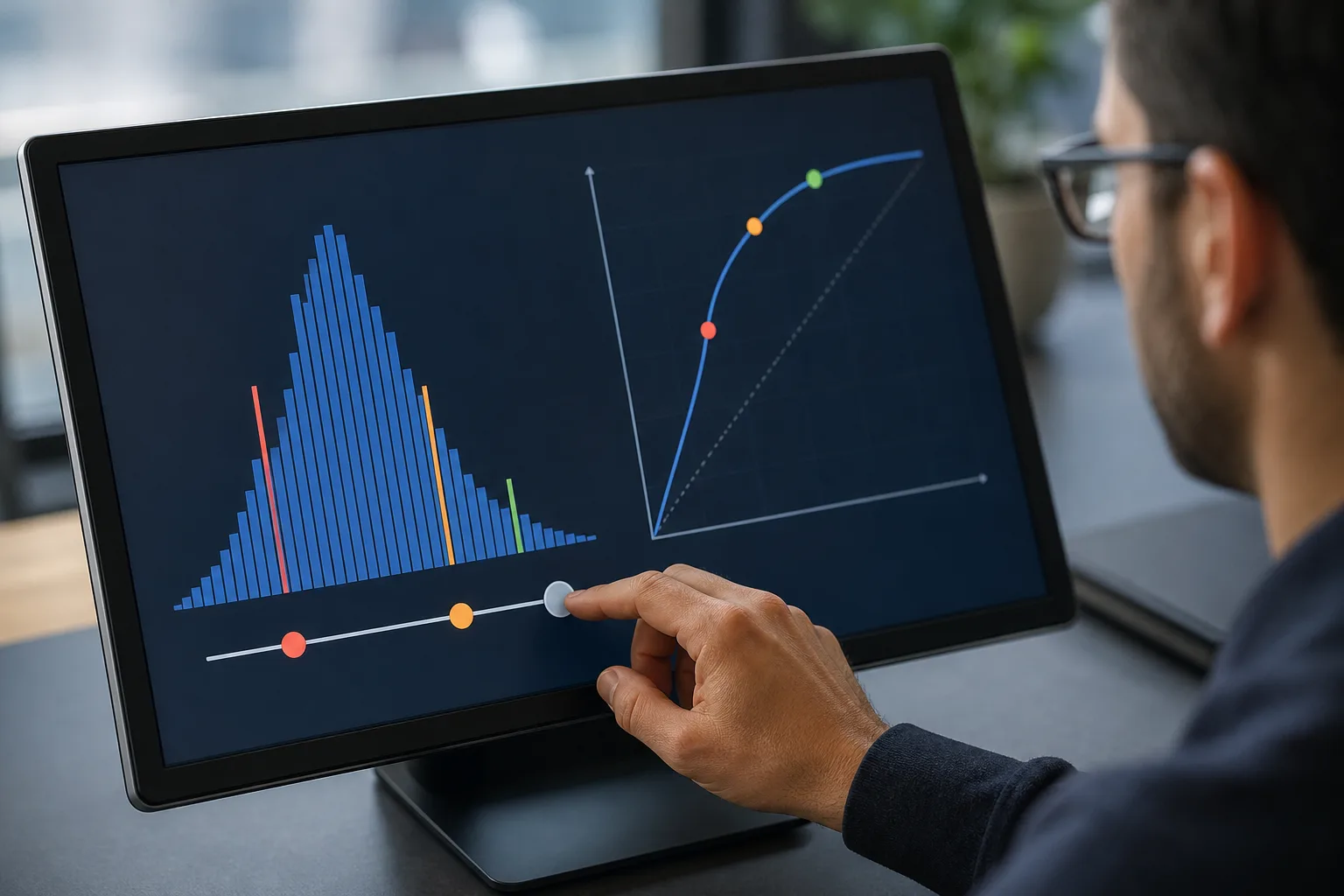
Each step adds a point to the curve. Connect the points and you have the ROC line. A curve that bows hard toward the top‑left is strong.
Step 3: Calculate AUC
Compute the area under that line. AUC = 0.5 means random. AUC = 1.0 means perfect ranking. Values like 0.70, 0.80, and 0.90 reflect better rank skill, but do not tell you the right threshold by themselves.
Step 4: Compare models
Plot several models on the same axes. If Model A’s curve is above Model B’s curve at most points, A ranks better. Use AUC as a quick tie‑breaker when curves cross. If two AUCs are close, look at the region that matters for your use case (for example, low‑FPR if false alarms are costly).
Step 5: Choose an optimal threshold
Pick a point on the curve that matches your costs. For fraud alerts, false alarms waste analyst time, so you might pick a low‑FPR point. For stroke screening, missing a case is worse, so you favor higher TPR even if FPR rises. You can use simple rules like Youden’s J (maximize TPR − FPR) as a starting point, then adjust with stakeholder input.
Visual cues to spot fast
- Steeper early rise (near FPR = 0): good at catching positives with few false alarms.
- Curve near diagonal: model adds little value; reconsider features or model type.
- Curves that cross: inspect your target operating zone, not just AUC.
Because this is a roc beginner guide roc, remember the goal: get a clear picture, then choose the threshold that serves your real costs, not a leaderboard.
Also Read!
Common Mistakes When Using ROC Curves
First, ignoring class imbalance. If positives are rare (say 1%), ROC can look fine even when most alerts are false. In that case, switch to a precision‑recall (PR) curve to see precision (of predicted positives, how many are real). Use ROC to judge ranking and PR to judge alert purity.
Second, confusing AUC with accuracy. A model can have strong AUC and weak accuracy at a bad cutoff. Flip it around: a model can look accurate on a skewed set by guessing the majority class, yet have poor AUC.
AUC measures ranking across all thresholds. Accuracy depends on one chosen threshold and class mix.
Third, evaluating only one threshold. Real systems drift. Costs shift. If you only check performance at 0.50, you may miss a better operating point at 0.72. Always scan the curve and review multiple cutoffs before you lock one in.
Fourth, assuming higher AUC always wins in the real world. If Model A has AUC 0.88 and Model B has 0.86, but B dominates in the low‑FPR region that you care about, B may be the smarter pick. Context beats a small AUC gap.
How to avoid these pitfalls
- Plot both ROC and PR when classes are imbalanced.
- Compare curves in the operating region that matches your costs.
- Re‑tune thresholds as data drifts; schedule reviews.
- Document your threshold choice and why it fits your risks.
A short note for this roc beginner guide roc: your stakeholders care about costs, not curves. Tie every chart back to missed‑case harm and false‑alarm waste.
Tools and Resources for Generating ROC Curves
You can generate ROC plots in most data stacks:
- scikit‑learn: Use functions like roc_curve and roc_auc_score to get points and AUC. Pair with matplotlib or seaborn to plot.
- R’s pROC package: Provides roc, auc, and smoothers, plus confidence intervals.
- TensorFlow Model Analysis: Computes ROC and AUC at scale on large evaluation slices.
From plots to production
After evaluation, you still need to ship. AI deployment services like GlobussoftAI OpenClaw Services can help teams move from a Jupyter plot to a live decision point with logs, alerts, and governance. The OpenClaw framework is free at its core, and a typical VPS costs around $5/month; total costs are usually under $10/month with AI model usage. That low base makes it practical to run ROC‑based monitors in production rather than leaving them on laptops.
Security and governance
As you scale, security matters. OpenClaw setups include end‑to‑end encryption and role‑based access controls to protect model outputs and audit trails.
For social proof, the OpenClaw ecosystem reached 100,000 GitHub stars in under eight weeks and drew on over 1,000 hours of testing data to explore what to automate. Those numbers show energy and care behind the tooling, which makes your 2027 deployment safer to operate.
“Businesses implementing AI services report up to a 40% reduction in operational costs and 30% increase in productivity.” — OpenClaw Services data
Moreover, the team offers AI/ML pipeline development for scalable deployment and model training and fine‑tuning on domain‑specific data, plus AI/ML consulting to build roadmaps and implement solutions. That means you can keep your ROC‑based checks close to the workflows they inform, not as side projects.
Key Takeaways

- ROC plots TPR vs FPR across thresholds; AUC sums ranking skill from 0.0 to 1.0.
- Choose thresholds based on business costs, not just the highest AUC.
- Use PR curves when classes are imbalanced or precision matters most.
- Compare curves in your operating zone; small AUC gaps can flip in practice.
- Ship your choice into production with security, logs, and routine re‑tuning.
What to Do Next: Putting ROC Analysis Into Practice
Set a one‑week plan to turn this roc beginner guide roc into action.
-
Pick a binary problem you know well. For example, “Will a transaction be disputed?” or “Is this email spam?” Export predicted scores and true labels on a held‑out test set.
-
Generate a ROC curve and AUC. In scikit‑learn, use roc_curve and roc_auc_score; in R, use pROC’s roc and auc. Save the plot and write down the AUC.
-
Compare two models. Train a simple baseline (like logistic regression) and a stronger model (like gradient boosting). Plot both curves together. Note where they cross and which one dominates in your low‑FPR or high‑TPR region.
-
Pick an operating threshold. Try Youden’s J (maximize TPR − FPR) as a start. Then adjust to hit a target like “no more than 5% false alarms.” Document the choice and why it fits your costs.
-
Research precision‑recall curves. If your positives are rare, add a PR plot and track precision at your chosen threshold. This guards against drowning your team in false alerts.
This week, move one step closer to a production‑ready decision. Save the plots, the AUC, and the chosen threshold in your project wiki with a clear note on the 2027 risks you’re managing. Then schedule a 30‑day check‑in to confirm the threshold still holds as data drifts.